Introduction
Materials and setup
Laptop users: you will need a copy of Stata installed on your machine. Harvard FAS affiliates can install a licensed version from http://downloads.fas.harvard.edu/download
- Find class materials at http://tutorials.iq.harvard.edu/Stata/StataIntro.zip
- Download and extract to your desktop!
Materials and setup
Laptop users: you will need a copy of Stata installed on your machine
Lab computer users: log in using your Athena user name and password
Everyone:
- Find class materials at http://tutorials.iq.harvard.edu/Stata/StataIntro.zip
- Download and extract to your desktop!
Organization
- Please feel free to ask questions at any point if they are relevant to the current topic (or if you are lost!)
- There will be a Q&A after class for more specific, personalized questions
- Collaboration with your neighbors is encouraged
- If you are using a laptop, you will need to adjust paths accordingly
- Make comments in your Do-file rather than on hand-outs
- save on flash drive or email to yourself
Workshop descripton
- This is an introduction to Stata
- Assumes no/very little knowledge of Stata
- Not appropriate for people already well familiar with Stata
- Learning Objectives:
- Familiarize yourself with the Stata interface
- Get data in and out of Stata
- Compute statistics and construct graphical displays
- Compute new variables and transformations
Why stata?
- Used in a variety of disciplines
- User-friendly
- Great guides available on web (as well as in HMDC computer lab library)
- Student and other discount packages available at reasonable cost
Stata interface
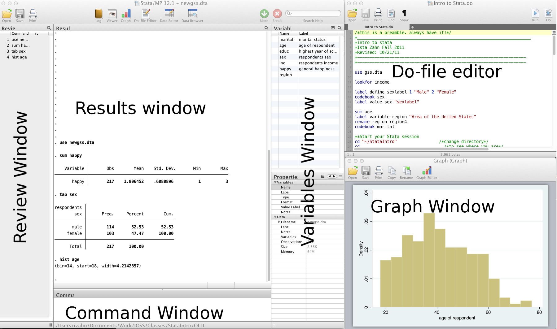
- Review and Variable windows can be closed (user preference)
- Command window can be shortened (recommended)
Do-files
- You can type all the same commands into the Do-file that you would type into the command window
- BUT...the Do-file allows you to save your commands
- Your Do-file should contain ALL commands you executed -- at least all the "correct" commands!
- I recommend never using the command window or menus to make CHANGES to data
- Saving commands in Do-file allows you to keep a written record of everything you have done to your data
- Allows easy replication
- Allows you to go back and re-run commands, analyses and make modifications
Stata help
To get help in Stata type help followed by topic or command, e.g., help codebook.
General Stata command syntax
Most Stata commands follow the same basic syntax: Command varlist, options.
Commenting and formatting syntax
Start with comment describing your Do-file and use comments throughout
* Use '*' to comment a line and '//' for in-line comments

* Make Stata say hello:
disp "Hello " "World!" // 'disp' is short for 'display'
- Use
///to break varlists over multiple lines:
disp "Hello" ///
     " World!"
Let's get started
- Launch the Stata program (MP or SE, does not matter unless doing computationally intensive work)
- Open up a new Do-file
- Run our first Stata code!
* change directory
// cd "C://Users/dataclass/Desktop/StataIntro"
cd dataSets

// open the gss.dta data set
use gss.dta, clear

// save data file:
save newgss.dta, replace // "replace" option means OK to overwrite existing file
A note about path names
- If your path has no spaces in the name (that means all directories, folders, file names, etc. can have no spaces), you can write the path as is
- If there are spaces, you need to put your pathname in quotes
- Best to get in the habit of quoting paths
Where's my data?
- Data editor (browse)
- Data editor (edit)
- Using the data editor is discouraged (why?)
- Always keep any changes to your data in your Do-file
- Avoid temptation of making manual changes by viewing data via the browser rather than editor
What if my data is not a Stata file?
- Import delimited text files
* import data from a .csv file
import delimited gss.csv, clear

* save data to a .csv file
export delimited gss_new.csv, replace
- Import data from SAS and Excel
* import/export SAS xport files
clear
import sasxport gss.xpt
export sasxport gss_new, replace
What if my data is from another statistical software program?
- SPSS/PASW will allow you to save your data as a Stata file
- Go to: file > save as > Stata (use most recent version available)
- Then you can just go into Stata and open it
- Another option is StatTransfer, a program that converts data from/to many common formats, including SAS, SPSS, Stata, and many more
Exercise 1: Importing data
- Save any work you've done so far. Close down Stata and open a new session.
- Start Stata and open your
.dofile. - Change directory (
cd) to thedataSetsfolder. - Try opening the following files:
- A comma separated value file: gss.csv
- An Excel file: gss.xlsx
Statistics and graphs
Frequently used commands
- Commands for reviewing and inspecting data:
- describe // labels, storage type etc.
- sum // statistical summary (mean, sd, min/max etc.)
- codebook // storage type, unique values, labels
- list // print actuall values
- tab // (cross) tabulate variables
- browse // view the data in a spreadsheet-like window
- Examples
use gss.dta, clear

sum educ // statistical summary of education
codebook region // information about how region is coded
tab sex // numbers of male and female participants
- If you run these commands without specifying variables, Stata will produce output for every variable
Basic graphing commands
- Univariate distribution(s) using hist
/* Histograms */
  hist educ
// histogram with normal curve; see 'help hist' for other options
  hist age, normal
- View bivariate distributions with scatterplots
/* scatterplots */
   twoway (scatter educ age)
graph matrix educ age inc
The "by" command
- Sometimes, you'd like to generate output based on different categories of a grouping variable
- The "by" command does just this
* By Processing
bysort sex: tab happy // tabulate happy separately for men and women
bysort marital: sum educ // summarize eudcation by marital status
Exercise 2: Descriptive statistics
- Use the dataset, gss.dta
- Examine a few selected variables using the describe, sum and codebook commands
- Tabulate the variable, "marital," with and without labels
- Summarize the variable, "income" by marital status
- Cross-tabulate marital with region
- Summarize the variable
happyfor married individuals only
Basic data management
Labels
- You never know why and when your data may be reviewed
- ALWAYS label every variable no matter how insignificant it may seem
- Stata uses two sets of labels: variable labels and value labels
- Variable labels are very easy to use -- value labels are a little more complicated
Variable and value labels
- Variable labels
/* Labelling and renaming */
  // Label variable inc "household income"
  label var inc "household income"

  // change the name 'educ' to 'education'
  rename educ education

  // you can search names and labels with 'lookfor'
  lookfor household
- Value labels are a two step process: define a value label, then assign defined label to variable(s)
/*define a value label for sex */
  label define mySexLabel 1 "Male" 2 "Female"
  /* assign our label set to the sex variable*/
  label val sex  mySexLabel
Exercise 3: Variable labels and value labels
- Open the data set gss.csv
- Familiarize yourself with the data using describe, sum, etc.
- Rename and label variables using the following codebook:
| var | rename to | label with |
|---|---|---|
| v1 | marital | marital status |
| v2 | age | age of respondent |
| v3 | educ | education |
| v4 | sex | respondent's sex |
| v5 | inc | household income |
| v6 | happy | general happiness |
| v7 | region | region of interview |
- Add value labels to your "marital" variable using this codebook:
| value | label |
|---|---|
| 1 | "married" |
| 2 | "widowed" |
| 3 | "divorced" |
| 4 | "separated" |
| 5 | "never married" |
Working on subsets
- It is often useful to select just those rows of your data where some condition holds--for example select only rows where sex is 1 (male)
- The following operators allow you to do this:
| Operator | Meaning |
|---|---|
| == | equal to |
| != | not equal to |
| > | greater than |
| >= | greater than or equal to |
| < | less than |
| <= | less than or equal to |
| & | and |
| or |
- Note the double equals signs for testing equality
Generating and replacing variables
- Create new variables using "gen"
// create a new variable named mc_inc
  //   equal to inc minus the mean of inc
  gen mc_inc = inc - 15.37
- Sometimes useful to start with blank values and fill them in based on values of existing variables
/* the 'generate and replace' strategy */
  // generate a column of missings
  gen age_wealth = .
  // Next, start adding your qualifications
  replace age_wealth=1 if age<30 & inc < 10
  replace age_wealth=2 if age<30 & inc > 10
  replace age_wealth=3 if age>30 & inc < 10
  replace age_wealth=4 if age>30 & inc > 10

  // conditions can also be combined with "or"
  gen young=0
  replace young=1 if age_wealth==1 | age_wealth==2
Exercise 4: Manipulating variables
- Use the dataset, gss.dta
- Generate a new variable, age2 equal to age squared
- Generate a new "high income" variable that will take on a value of "1" if a person has an income value greater than "15" and "0" otherwise
- Generate a new divorced/separated dummy variable that will take on a value of "1" if a person is either divorced or separated and "0" otherwise
Wrap-up
Help us make this workshop better!
Please take a moment to fill out a very short feedback form
These workshops exist for you – tell us what you need!
Additional resources
IQSS workshops: http://projects.iq.harvard.edu/rtc/filter_by/workshops
IQSS statistical consulting: http://dss.iq.harvard.edu
The RCE
- Research Computing Enviroment (RCE) service available to Harvard & MIT users
- http://www.iq.harvard.edu/research_computing
- Wonderful resource for organizing data, running analyses efficiently
- Creates a centralized place to store data and run analysis
- Supplies persistent desktop environment accessible from any computer with an internet connection