Large Data in R: Tools and Techniques

Set Up and Example Data

The examples and exercises require R and several R packages, including tidyverse, data.table, arrow, and duckdb. This software is all installed and ready to use on the HBS Grid. If running elsewhere make sure these required software programs are installed before proceeding.

You can download and extract the data used in the examples and exercises from https://www.dropbox.com/s/vbodicsu591o7lf/original_csv.zip?dl=1 (this is a 1.3Gb zip file). These data record for-hire vehicle (aka “ride sharing”) trips in NYC in 2020. Each row contains the record of a trip and the variable descriptions can be found in https://www1.nyc.gov/assets/tlc/downloads/pdf/data_dictionary_trip_records_hvfhs.pdf

Nature and Scope of the Problem: What is Large Data?

Most popular data analysis software is designed to operate on data stored in random access memory (aka just “memory” or “RAM”). This makes modifying and copying data very fast and convenient, until you start working with data that is too large for your computer’s memory system. At that point you have two options: get a bigger computer or modify your workflow to process the data more carefully and efficiently. This workshop focuses on option two, using the arrow and duckdb packages in R to work with data without necessarily loading it all into memory at once.

A common definition of “big data” is “data that is too big to process using traditional software”. We can use the term “large data” as a broader category of “data that is big enough that you have to pay attention to processing it efficiently”.

In a typical (traditional) program, we start with data on disk, in some format. We read it in to memory, do some stuff to it on the CPU, store the results of that stuff back in memory, then write those results back to disk so they can be available for the future, as depicted below.

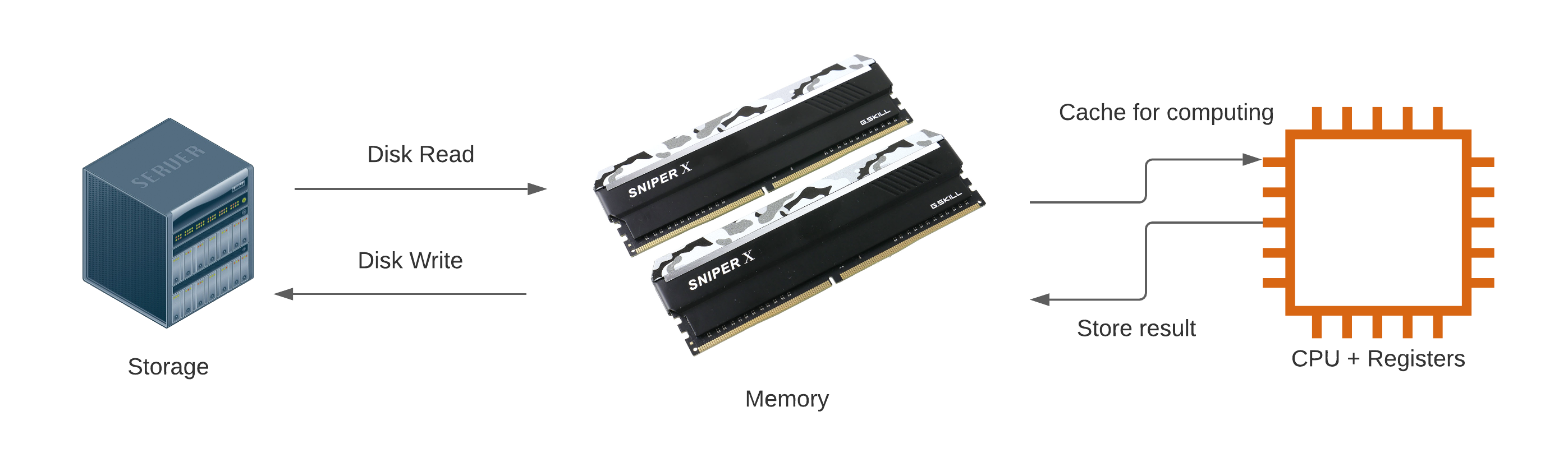Flow of Data in A Program The reason most data analysis software is designed to process data this way is because “doing some stuff” is much much faster in RAM than it is if you have to read values from disk every time you need them. The downside is that RAM is much more expensive than disk storage, and typically available in smaller quantities. Memory can only hold so much data and we must either stay under that limit or buy more memory.

Problem example

Grounding our discussion in a concrete problem example will help make things clear. I want to know how many Lyft rides were taken in New York City during 2020. The data is publicly available as documented at https://www1.nyc.gov/site/tlc/about/tlc-trip-record-data.page and I have made a subset available on dropbox as described in the Setup section above for convenience. Documentation can be found at https://www1.nyc.gov/assets/tlc/downloads/pdf/data_dictionary_trip_records_hvfhs.pdf

In order to demonstrate large data problems and solutions I’m going to artificially limit my system to 4Gb of memory. This will allow us to quickly see what happens when we reach the memory limit, and to look at solutions to that problem without waiting for our program to read in hundreds of Gb of data. (There is no need to follow along with this step, the purpose is just to make sure we all know what happens when you run out of memory.)

Start by looking at the file names and sizes:

fhvhv_csv_files <- list.files("original_csv", recursive=TRUE, full.names = TRUE)
data.frame(file = fhvhv_csv_files, size_Mb = file.size(fhvhv_csv_files) / 1024^2)

##                                               file   size_Mb
## 1  original_csv/2020/01/fhvhv_tripdata_2020-01.csv 1243.4975
## 2  original_csv/2020/02/fhvhv_tripdata_2020-02.csv 1313.2442
## 3  original_csv/2020/03/fhvhv_tripdata_2020-03.csv  808.5597
## 4  original_csv/2020/04/fhvhv_tripdata_2020-04.csv  259.5806
## 5  original_csv/2020/05/fhvhv_tripdata_2020-05.csv  366.5430
## 6  original_csv/2020/06/fhvhv_tripdata_2020-06.csv  454.5977
## 7  original_csv/2020/07/fhvhv_tripdata_2020-07.csv  599.2560
## 8  original_csv/2020/08/fhvhv_tripdata_2020-08.csv  667.6880
## 9  original_csv/2020/09/fhvhv_tripdata_2020-09.csv  728.5463
## 10 original_csv/2020/10/fhvhv_tripdata_2020-10.csv  798.4743
## 11 original_csv/2020/11/fhvhv_tripdata_2020-11.csv  698.0638
## 12 original_csv/2020/12/fhvhv_tripdata_2020-12.csv  700.6804

We can already guess based on these file sizes that with only 4 Gb of RAM available we’re going to have a problem.

library(tidyverse)
fhvhv_data <- map(fhvhv_csv_files, read_csv) %>% bind_rows(show_col_types=FALSE)

## Error in eval(expr, envir, enclos): cannot allocate vector of size 7.6 Mb

Perhaps you’ve seen similar messages before. Basically it means that we don’t have enough memory available to hold the data we want to work with. I previously ran the code chunk above with more memory and found that it required just over 16 Gb. How can we work with data when we only have 1/4 of the memory requirement available?

The Evergiven An example of a large object causing a bottleneck

General strategies and principles

Part of the problem with our first attempt is that CSV files do not make it easy to quickly read subsets or select columns. In this section we’ll spend some time identifying strategies for working with large data and identify some tools that make it easy to implement those strategies.

Use a fast binary data storage format that enables reading data subsets

CSVs, TSVs, and similar delimited files are all text-based formats that are typically used to store tabular data. Other more general text-based data storage formats are in wide use as well, including XML and JSON. These text-based formats have the advantage of being both human and machine readable, but text is a relatively inefficient way to store data, and loading it into memory requires a time-consuming parsing process to separate out the fields and records.

As an alternative to text-based data storage formats, binary formats have the advantage of being more space efficient on disk and faster to read. They often employ advanced compression techniques, store metadata, and allow fast selective access to data subsets. These substantial advantages come at the cost of human readability; you cannot easily inspect the contents of binary data files directly. If you are concerned with reducing memory use or data processing time this is probably a trade-off you are happy to make.

The parquet binary storage format is among the best currently available. Support in R is provided by the arrow package. In a moment we’ll see how we can use the arrow package to dramatically reduce the time it takes to get data from disk to memory and back.

Partition the data on disk to facilitate chunked access and computation

Memory requirements can be reduced by partitioning the data and computation into chunks, running each one sequentially, and combining the results at the end. It is common practice to partition the data on disk storage to make this computational strategy more natural and efficient. For example, the taxi data is already partitioned by year and month.

Only read in the data you need

If we think carefully about it we’ll see that our previous attempt to process the taxi data by reading in all the data at once was wasteful. Not all the rows are Lyft rides, and the only column I really need is the one that tells me if the ride was operated by Lyft or not. I can perform the computation I need by only reading in that one column, and only the rows for which the hvfhs_license_num column is equal to HV0005 (Lyft).

Use streaming data tools and algorithms

It’s all fine and good to say “only read the data you need”, but how do you actually do that? Unless you have full control over the data collection and storage process, chances are good that your data provider included a bunch of stuff you don’t need. The key is to find a data selection and filtering tool that works in a streaming fashion so that you can access subsets without ever loading data you don’t need into memory. Both the arrow and duckdb R packages support this type of workflow and can dramatically reduce the time and hardware requirements for many computations.

Moreover, processing data in a streaming fashion without needing to load it into memory is a general technique that can be applied to other tasks as well. For example the duckdb package allows you to carry out data aggregation in a streaming fashion, meaning that you can compute summary statistics for data that is too large to fit in memory.

Avoid unnecessarily storing or duplicating data in memory

It is also important to pay some attention to storing and processing data efficiently once we have it loaded in memory. R likes to make copies of the data, and while it does try to avoid unnecessary duplication this process can be unpredictable. At a minimum you can remove or avoid storing intermediate results you don’t need and take care not to make copies of your data structures unless you have to. The data.table package additionally makes it easier to efficiently modify R data objects in-place, reducing the risk of accidentally or unknowingly duplicating large data structures.

Technique summary

We’ve accumulated a list of helpful techniques! To review:

Use a fast binary data storage format that enables reading data subsets
Partition the data on disk to facilitate chunked access and computation
Only read in the data you need
Use streaming data tools and algorithms
Avoid unnecessarily storing or duplicating data in memory

Solution example

Now that we have some theoretical foundations to build on we can start putting these techniques into practice. Using the techniques identified above will allow us to overcome the memory limitation we ran up against before, and finally answer the question “How many Lyft rides were taken in New York City during 2020?”?

Convert .csv to parquet

The first step is to take the slow and inefficient text-based data provided by the city of New York and convert it to parquet using the arrow package. This is a one-time up-front cost that may be expensive in terms of time and/or computational resources. If you plan to work with the data a lot it will be well worth it because it allows subsequent reads to be faster and more memory efficient.

library(arrow)

if(!dir.exists("converted_parquet")) {

  dir.create("converted_parquet")

  ## this doesn't yet read the data in, it only creates a connection
  csv_ds <- open_dataset("original_csv", 
                         format = "csv",
                         partitioning = c("year", "month"))

  ## this reads each csv file in the csv_ds dataset and converts it to a .parquet file
  write_dataset(csv_ds, 
                "converted_parquet", 
                format = "parquet",
                partitioning = c("year", "month"))
}

This conversion is relatively easy (even with limited memory) because the data provider is already using one of our strategies, i.e., they partitioned the data by year/month. This allows us to convert each file one at a time, without ever needing to read in all the data at once.

We also took care to preserve the year/month partition into sub-directories. We improved on the implementation by using what is known as “hive-style” partitioning, i.e., including both the variable names and values in the directory names. This is convenient because it makes it easy for arrow (and other tools that recognize the hive partitioning standard) to automatically recognize the partitions.

We can look at the converted files and compare the naming scheme and storage requirements to the original CSV data.

fhvhv_csv_files <- list.files("original_csv", recursive=TRUE, full.names = TRUE)
fhvhv_files <- list.files("converted_parquet", full.names = TRUE, recursive = TRUE)

data.frame(csv_file = fhvhv_csv_files, 
           parquet_file = fhvhv_files, 
           csv_size_Mb = file.size(fhvhv_csv_files) / 1024^2, 
           parquet_size_Mb = file.size(fhvhv_files) / 1024^2)

                                                                 CSV        Parquet
                  csv_file                       parquet_file    size_Mb    size_Mb
fhvhv_tripdata_2020-01.csv   year=2020/month=1/part-0.parquet  1243.4975  190.26387
fhvhv_tripdata_2020-02.csv  year=2020/month=10/part-0.parquet  1313.2442  125.17837
fhvhv_tripdata_2020-03.csv  year=2020/month=11/part-0.parquet   808.5597  110.92144
fhvhv_tripdata_2020-04.csv  year=2020/month=12/part-0.parquet   259.5806  111.67697
fhvhv_tripdata_2020-05.csv   year=2020/month=2/part-0.parquet   366.5430  198.87074
fhvhv_tripdata_2020-06.csv   year=2020/month=3/part-0.parquet   454.5977  127.53637
fhvhv_tripdata_2020-07.csv   year=2020/month=4/part-0.parquet   599.2560   48.32047
fhvhv_tripdata_2020-08.csv   year=2020/month=5/part-0.parquet   667.6880   64.17768
fhvhv_tripdata_2020-09.csv   year=2020/month=6/part-0.parquet   728.5463   76.45972
fhvhv_tripdata_2020-10.csv   year=2020/month=7/part-0.parquet   798.4743   97.99151
fhvhv_tripdata_2020-11.csv   year=2020/month=8/part-0.parquet   698.0638  107.80694
fhvhv_tripdata_2020-12.csv   year=2020/month=9/part-0.parquet   700.6804  115.25221

As expected, the binary parquet storage format is much more compact than the text-based CSV format. This is one reason that reading parquet data is so much faster:

## tidyverse csv reader
system.time(invisible(readr::read_csv(fhvhv_csv_files[[1]], show_col_types = FALSE)))

##    user  system elapsed 
##  79.982   6.362  31.824

## arrow package parquet reader
system.time(invisible(read_parquet(fhvhv_files[[1]])))

##    user  system elapsed 
##   5.761   2.226  22.533

Read and count Lyft records with arrow

The arrow package makes it easy to read and process only the data we need for a particular calculation. It allows us to use the partitioned data directories we created earlier as a single dataset and to query it using the dplyr verbs many R users are already familiar with.

Start by creating a dataset representation from the partitioned data directory:

fhvhv_ds <- open_dataset("converted_parquet",
                         schema = schema(hvfhs_license_num=string(),
                                         dispatching_base_num=string(),
                                         pickup_datetime=string(),
                                         dropoff_datetime=string(),
                                         PULocationID=int64(),
                                         DOLocationID=int64(),
                                         SR_Flag=int64(),
                                         year=int32(),
                                         month=int32()))

Because we have hive-style directory names open_dataset automatically recognizes the partitions. Note that usually we do not need to manually specify the schema, we do so here to work around an issue with duckdb support.

Importantly, open_dataset doesn’t actually read the data into memory. It just opens a connection to the dataset and makes it easy for us to query it. Finally, we can compute the number of NYC Lyft trips in 2020, even on a machine with limited memory:

library(dplyr, warn.conflicts = FALSE)

fhvhv_ds %>%
  filter(hvfhs_license_num == "HV0005") %>%
  select(hvfhs_license_num) %>%
  collect() %>%
  summarize(total_Lyft_trips = n())

## # A tibble: 1 × 1
##   total_Lyft_trips
##              <int>
## 1         37250101

Note that arrow datasets do not support summarize natively, that is why we call collect first to actually read in the data.

The arrow package makes it fast and easy to query on-disk data and read in only the fields and records needed for a particular computation. This is a tremendous improvement over the typical R workflow, and may well be all you need to start using your large datasets more quickly and conveniently, even on modest hardware.

Efficiently query taxi data with duckdb

If you need even more speed and convenience you can use the duckdb package. It allows you to query the same parquet datasets partitioned on disk as we did above. You can use either SQL statements via the DBI package or tidyverse style verbs using dbplyr. Let’s see how it works.

First we create a duckdb table from our arrow dataset.

library(duckdb)
library(dplyr)

con <- DBI::dbConnect(duckdb::duckdb())
fhvhv_tbl <- to_duckdb(fhvhv_ds, con, "fhvhv")

The duckdb table can be queried using tidyverse style verbs or SQL.

## number of Lyft trips, tidyverse style
fhvhv_tbl %>%
  filter(hvfhs_license_num == "HV0005") %>%
  select(hvfhs_license_num) %>%
  count()

## # Source:   lazy query [?? x 1]
## # Database: duckdb_connection
##          n
##      <dbl>
## 1 37250101

## number of Lyft trips, SQL style
y <- dbSendQuery(con, "SELECT COUNT(*) FROM fhvhv WHERE hvfhs_license_num=='HV0005';")
dbFetch(y)

##   count_star()
## 1     37250101

The main advantages of duckdb are that it has full SQL support, supports aggregating data in a streaming fashion, allows you to set memory limits, and is optimized for speed. The way I think about the relationship between arrow and duckdb is that arrow is primarily about reading and writing data as fast and efficiently as possible, with some built-in analysis capabilities, while duckdb is a database engine with more complete data manipulation and aggregation capabilities.

It can be instructive to compare arrow and duckdb capabilities and performance using a slightly more complicated example. Here we compute a grouped average using arrow:

system.time({fhvhv_ds %>%
    filter(hvfhs_license_num == "HV0005") %>%
    select(hvfhs_license_num, month) %>%
    group_by(hvfhs_license_num) %>%
    collect() %>%
    summarize(avg = mean(month, na.rm = TRUE)) %>%
    print()})

## # A tibble: 1 × 2
##   hvfhs_license_num   avg
##   <chr>             <dbl>
## 1 HV0005             6.10

##    user  system elapsed 
##  19.456   4.064  14.254

note that we use collect to read the data into memory before the summarize step because arrow does not support aggregating in a streaming fashion.

Here is the same query using duckdb:

system.time({fhvhv_tbl %>%
    filter(hvfhs_license_num == "HV0005") %>%
    select(hvfhs_license_num, month) %>%
    group_by(hvfhs_license_num) %>%
    summarize(avg = mean(month, na.rm = TRUE)) %>%
    print()})

## # Source:   lazy query [?? x 2]
## # Database: duckdb_connection
##   hvfhs_license_num   avg
##   <chr>             <dbl>
## 1 HV0005             6.10

##    user  system elapsed 
##  18.766   1.251   8.984

note that it is slightly faster, and we don’t need to read as much data into memory because duckdb supports aggregating in a streaming fashion. This capability is very powerful because it allows us to perform computations on data that is too big to fit into memory.

Your turn!

Now that you understand some of the basic techniques for working with large data and have seen an example, you can start to apply what you’ve learned. Using the same taxi data, try answering the following questions:

What percentage of trips are made by Lyft?
In which month did Lyft log the most trips?

Documentation for these data can be found at https://www1.nyc.gov/assets/tlc/downloads/pdf/data_dictionary_trip_records_hvfhs.pdf