Programming with Databases - R

Overview

Teaching: 30 min
Exercises: 15 min

Questions

How can I access databases from programs written in R?

Objectives

Write short programs that execute SQL queries.

Trace the execution of a program that contains an SQL query.

Explain why most database applications are written in a general-purpose language rather than in SQL.

To close, let’s have a look at how to access a database from a data analysis language like R. Other languages use almost exactly the same model: library and function names may differ, but the concepts are the same.

Here’s a short R program that selects latitudes and longitudes from an SQLite database stored in a file called survey.db:

library(RSQLite)
connection <- dbConnect(SQLite(), "survey.db")
results <- dbGetQuery(connection, "SELECT Site.lat, Site.long FROM Site;")
print(results)
dbDisconnect(connection)

     lat    long
-49.85 -128.57
-47.15 -126.72
-48.87 -123.40

The program starts by importing the RSQLite library. If we were connecting to MySQL, DB2, or some other database, we would import a different library, but all of them provide the same functions, so that the rest of our program does not have to change (at least, not much) if we switch from one database to another.

Line 2 establishes a connection to the database. Since we’re using SQLite, all we need to specify is the name of the database file. Other systems may require us to provide a username and password as well.

On line 3, we retrieve the results from an SQL query. It’s our job to make sure that SQL is properly formatted; if it isn’t, or if something goes wrong when it is being executed, the database will report an error. This result is a dataframe with one row for each entry and one column for each column in the database.

Finally, the last line closes our connection, since the database can only keep a limited number of these open at one time. Since establishing a connection takes time, though, we shouldn’t open a connection, do one operation, then close the connection, only to reopen it a few microseconds later to do another operation. Instead, it’s normal to create one connection that stays open for the lifetime of the program.

Queries in real applications will often depend on values provided by users. For example, this function takes a user’s ID as a parameter and returns their name:

library(RSQLite)

connection <- dbConnect(SQLite(), "survey.db")

getName <- function(personID) {
  query <- paste0("SELECT personal || ' ' || family FROM Person WHERE id =='",
                  personID, "';")
  return(dbGetQuery(connection, query))
}

print(paste("full name for dyer:", getName('dyer')))

dbDisconnect(connection)

full name for dyer: William Dyer

We use string concatenation on the first line of this function to construct a query containing the user ID we have been given. This seems simple enough, but what happens if someone gives us this string as input?

dyer'; DROP TABLE Survey; SELECT '

It looks like there’s garbage after the user’s ID, but it is very carefully chosen garbage. If we insert this string into our query, the result is:

SELECT personal || ' ' || family FROM Person WHERE id='dyer'; DROP TABLE Survey; SELECT '';

If we execute this, it will erase one of the tables in our database.

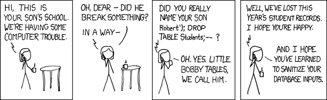
This is called an SQL injection attack, and it has been used to attack thousands of programs over the years. In particular, many web sites that take data from users insert values directly into queries without checking them carefully first. A very relevant XKCD that explains the dangers of using raw input in queries a little more succinctly:

relevant XKCD

Since an unscrupulous parent might try to smuggle commands into our queries in many different ways, the safest way to deal with this threat is to replace characters like quotes with their escaped equivalents, so that we can safely put whatever the user gives us inside a string. We can do this by using a prepared statement instead of formatting our statements as strings. Here’s what our example program looks like if we do this:

library(RSQLite)
connection <- dbConnect(SQLite(), "survey.db")

getName <- function(personID) {
  query <- "SELECT personal || ' ' || family FROM Person WHERE id == ?"
  return(dbGetPreparedQuery(connection, query, data.frame(personID)))
}

print(paste("full name for dyer:", getName('dyer')))

dbDisconnect(connection)

full name for dyer: William Dyer

The key changes are in the query string and the dbGetQuery call (we use dbGetPreparedQuery instead). Instead of formatting the query ourselves, we put question marks in the query template where we want to insert values. When we call dbGetPreparedQuery, we provide a dataframe that contains as many values as there are question marks in the query. The library matches values to question marks in order, and translates any special characters in the values into their escaped equivalents so that they are safe to use.

Filling a Table vs. Printing Values

Write an R program that creates a new database in a file called original.db containing a single table called Pressure, with a single field called reading, and inserts 100,000 random numbers between 10.0 and 25.0. How long does it take this program to run? How long does it take to run a program that simply writes those random numbers to a file?

Filtering in SQL vs. Filtering in R

Write an R program that creates a new database called backup.db with the same structure as original.db and copies all the values greater than 20.0 from original.db to backup.db. Which is faster: filtering values in the query, or reading everything into memory and filtering in R?

Database helper functions in R

R’s database interface packages (like RSQLite) all share a common set of helper functions useful for exploring databases and reading/writing entire tables at once.

To view all tables in a database, we can use dbListTables():

connection <- dbConnect(SQLite(), "survey.db")
dbListTables(connection)

"Person"  "Site"    "Survey"  "Visited"

To view all column names of a table, use dbListFields():

dbListFields(connection, "Survey")

"visited_id"   "person_id"  "quant"   "reading"

To read an entire table as a dataframe, use dbReadTable():

dbReadTable(connection, "Person")

        id  personal   family
   dyer   William     Dyer
     pb     Frank  Pabodie
   lake  Anderson     Lake
    roe Valentina  Roerich
danforth     Frank Danforth

Finally to write an entire table to a database, you can use dbWriteTable(). Note that we will always want to use the row.names = FALSE argument or R will write the row names as a separate column. In this example we will write R’s built-in iris dataset as a table in survey.db.

dbWriteTable(connection, "iris", iris, row.names = FALSE)
head(dbReadTable(connection, "iris"))

  Sepal.Length Sepal.Width Petal.Length Petal.Width Species
        5.1         3.5          1.4         0.2  setosa
        4.9         3.0          1.4         0.2  setosa
        4.7         3.2          1.3         0.2  setosa
        4.6         3.1          1.5         0.2  setosa
        5.0         3.6          1.4         0.2  setosa
        5.4         3.9          1.7         0.4  setosa

And as always, remember to close the database connection when done!

dbDisconnect(connection)

R and dplyr / dbplyr

We’re going to try a different approach, one that does not use explicit SQL statements and instead uses the more natural syntax of R and dplyr. But we’ll show you the comparisons. You can download R_sqlite_dplyr.R to your local machine and put it in your Desktop/ folder.

Setup: Some initial configuration is needed:

## let's ensure that we have the correct packages loaded
# and set the appropriate working directory
install.packages(c("RSQLite", "dplyr", "dbplyr"))
setwd("/Users/(your_username)/Desktop/")

If all goes well, we can proceed…

Standard R and SQL: We’ll issue an SQL statement to the database in R to gather our data:

### Standard SQL
# import our required packages
library('RSQLite')

# open the database connection
connection <- dbConnect(SQLite(), "survey.db")

# execute and fetch the results
results <- dbGetQuery(connection, "SELECT Site.lat, Site.long FROM Site;")

# print 'em out
print(results)

# close the connection
dbDisconnect(connection)

Well, that was fun. But let’s do it a little differently…

R with dplyr: Let’s use dplyr verbs to work with our data and the database, but we are still doing SQL:

### Somewhat using dplyr
# import our required packages
library('dplyr')

# create connection with RSQLite driver
connection <- DBI::dbConnect(RSQLite::SQLite(), "survey.db")

# execute and fetch the results
results <- tbl(connection, sql("SELECT Site.lat, Site.long FROM Site"))

# print 'em out & close connection
print(results)
DBI::dbConnect(connection)

You’ll notie the results are somewhat truncated (we’re working on this). But we have them just the same.

R with dplyr and dbplyr: Now let’s show SQL vs dplyr verbs:

### Real dplyr with dbplyr
#
library(dplyr)
library(dbplyr)

# open a connection and give us information about it
connection <- DBI::dbConnect(RSQLite::SQLite(), "survey.db")
src_dbi(connection)

# SQL approach, seeing what the data is and the data structure (messy)
results <- tbl(connection, sql("SELECT Site.lat, Site.long FROM Site"))
results
str(results)

# dplyr approach, see data structure and use pipes
sites <- tbl(connection, "Site")
str(sites)
sites %>% 
  select(lat, long)

# see the SQL generated and disconnect
sites %>% 
  select(lat, long) %>%
  show_query()
DBI::dbDisconnect(connection)

Here we used native dplyr vers to specify the table and to filter data. Much nicer! And we can continue with more complex queries:

## Simple query and filter
#
# find readings out of range:
# SELECT * FROM Survey WHERE quant = 'sal' AND ((reading > 1.0) OR (reading < 0.0));


connection <- DBI::dbConnect(RSQLite::SQLite(), "survey.db")
src_dbi(connection)

# now do our query...
survey <- tbl(connection, "Survey")
survey %>% 
  select(person_id, quant, reading) %>% 
  filter(quant == 'sal',
         reading > 1 | reading < 0)

# what did it do? show us the SQL
survey %>% 
  select(person_id, quant, reading) %>% 
  filter(quant == 'sal',
         reading > 1 | reading < 0) %>% 
  show_query()

# collect our data, print it, and disconnect
salinity_readings <- survey %>% 
  select(person_id, quant, reading) %>% 
  filter(quant == 'sal',
         reading > 1 | reading < 0)
salinity_readings
DBI::dbDisconnect(connection)

Wow! Isn’t that nice? Let’s try a join:

## Do a join
#
# SELECT * FROM Visited JOIN Survey 
# ON Survey.taken = Visited.id and person = "lake" ORDER BY quant ASC;

library(dplyr)
library(dbplyr)

connection <- DBI::dbConnect(RSQLite::SQLite(), "survey.db")
src_dbi(connection)

# now join Survey to other table Visit, identifying ties, then continue filter...
survey <- tbl(connection, "Survey")
both <- left_join(survey, tbl(connection, "Visited"),
                   by = c("visited_id" = "id")) %>% 
  filter(person_id == "lake") %>%
  arrange(quant)
both

# tell us what happened, and exit
explain(both)
DBI::dbDisconnect(connection)

We hope that you see that using native R dplyr syntax is much easier and more natural than explicit SQL queries for routine and lightweight work. Feel free to explore the documentation for dply and dbplyr.

Key Points

Data analysis languages have libraries for accessing databases.

To connect to a database, a program must use a library specific to that database manager.

R’s libraries can be used to directly query or read from a database.

Programs can read query results in batches or all at once.

Queries should be written using parameter substitution, not string formatting.

R has multiple helper functions to make working with databases easier.

previous episode

Databases and SQL

lesson home

Programming with Databases - R

Overview

Filling a Table vs. Printing Values

Filtering in SQL vs. Filtering in R

Database helper functions in R

R and dplyr / dbplyr

Key Points

previous episode

lesson home